


Over the last two decades, there have been tremendous advances in quantum Monte Carlo (QMC) methods, such as the development of the Stochastic Series Expansion (Sandvik) and the loop algorithm (Evertz), and in Dynamical Mean Field theory (Jarrell, Georges, Kotliar, ...). These advances have opened new frontiers in our understanding of quantum phase transitions. I have developed a quantum Monte Carlo method, the Stochastic Green Function (SGF) algorithm, which opens the way to the exact simulation of Hamiltonians with high order terms (for example, Hamiltonians with six-site coupling terms).
Here is a list of the main properties of the algorithm:
This is a question that is often asked, and the answer naturally comes when one tries to use other algorithms to simulate a Hamiltonian like this (consider a two-dimensional kagome lattice):
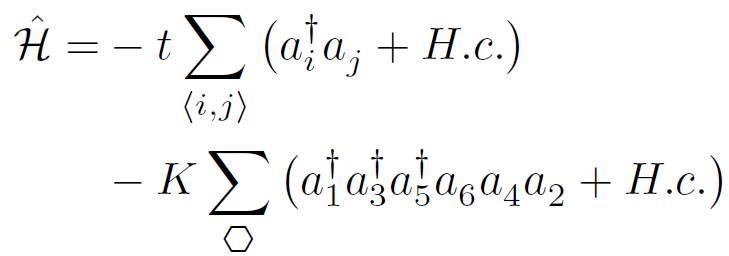
To be honest, trying to simulate this Hamiltonian with other algorithms gives terrible headaches, because of the sixth order interaction term! The reason is that other algorithms normally need to decompose the Hamiltonian as a sum of two-site problems, which in the above example is impossible. There exists some non-trivial extensions that allow those algorithms to treat fourth order terms in some particular cases, but generalizing these to any Hamiltonian is cumbersome (if not impossible).
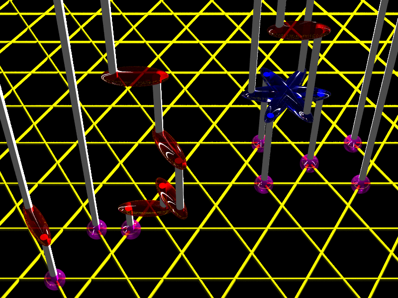
So the answer to the question is “yes, SGF is different from other algorithms”, and the proof is that simulating the above Hamiltonian with SGF is straightforward! This is because the SGF algorithm does not require any special decomposition of the Hamiltonian. It performs a direct sampling of the partition function by distributing Hamiltonian terms at random (with importance sampling) in imaginary time. Thus, the algorithm is completely independent of the structure of the Hamiltonian. The figure below shows an example of a configuration that can be generated. The yellow lines represent the structure of the lattice. The imaginary time axis is perpendicular to the lattice plane. An initial state for the particles (purple spheres) is chosen at imaginary time τ=0. As the imaginary time increases, some Hamiltonian terms are distributed. The red ellipsoids represent kinetic terms, and the blue star represents a ring-exchange term that performs a correlated hopping of three particles at the same time. The gray lines are the worldlines of the particles.
The SGF algorithm performs a stochastic expansion of the partition function, but not the same as in the Stochastic Series Expansion (SSE) algorithm. Actually, SGF and SSE are totally different:
SGF is actually derived from the Worm algorithm in its canonical implementation:
However, the extended space visited by the SGF algorithm is different, as well as the global update procedure. And it is precisely these differences that allow to easily simulate any Hamiltonian in both the canonical and the grand-canonical ensembles. The SGF global update procedure does not need to make any assumption on the Hamiltonian that is simulated. It is totally independent of the Hamiltonian, thus a single computer code is able to simulate any Hamiltonian with no other modifications than the list of Hamiltonian terms.
Another difference between the SGF algorithm and the Worm algorithm in its canonical implementation is that it is necessary for the latter to reject some of the updates in order to satisfy detailed balance (except for some particular Hamiltonians). This introduces some complexity in the update procedure because one needs to keep track of the history of the update in case of a rejection. This also slows down the simulation since the time spent on a rejected update is wasted. Moreover, the ergodicity is not garanteed when systematic rejections occur. With the SGF algorithm, however, the acceptance rate of the updates is 100% for any Hamiltonian ensuring efficiency and simplicity!
The SGF algorithm directly operates in second quantization. So we start by choosing an occupation number basis. Once the basis is chosen, the Hamiltonian is written as a diagonal operator V minus a non-diagonal operator T:

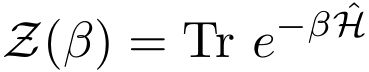
This is the only decomposition that needs to be performed, and this decomposition is obviously always possible (while other algorithms need to make more assumptions on the form of the Hamiltonian). The purpose is to sample the partition function:
To this end, we define the Green operator G by its matrix elements for all pairs of states ψL and ψR,
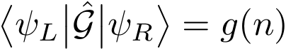
where g is a decreasing function of the number n of creations and annihilations that connect the two states. By breaking up the propagator at imaginary time τ and introducing the Green operator between the two parts, we can define an “extended partition function”:
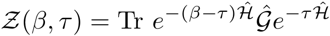
Defining the time dependence of T(τ) and G(τ) in the interaction picture, the extended partition function can be expanded as:
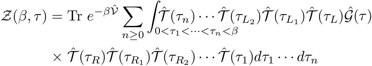
Note that we have used the labels L, L1, L2, ... (resp. R, R1, R2, ...) to denote the first, second, third, ... time indices that appear on the left (resp. right) of the Green operator. Finally, by introducing n complete sets of states and writing explicitly the trace, the partition function takes the form:
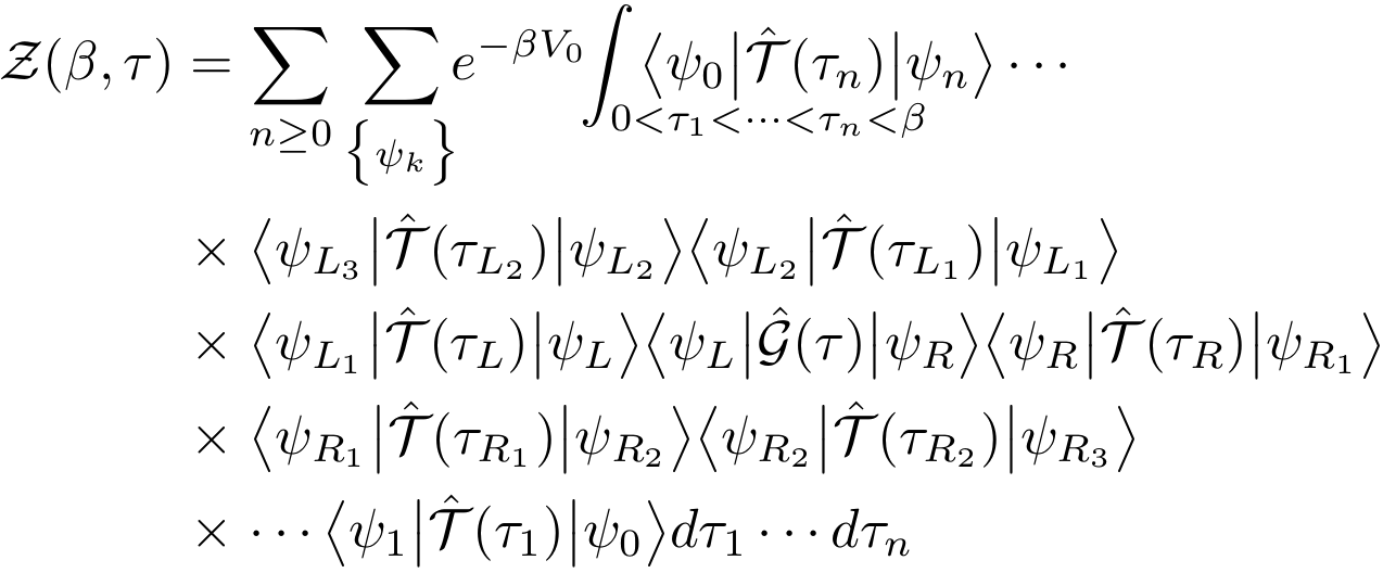
We have used the notation V0 for the eigenvalue of V with the eigenstate ψ0. Thus, the extended partition function is the sum over all possible strings of T operators. The purpose of the algorithm is to generate those operator strings with the Boltzmann weight. In order to achieve this, the Green operator is propagated in imaginary time to the left (increasing time) or to the right (decreasing time). While propagating, the Green operator can create a T operator or destroy a T operator that is encountered:


An efficient way to do this is to use the update scheme depicted in the figure below. A direction of propagation to the left or to the right is chosen for the Green operator. Then an action, creation or destruction, is chosen. If creation is chosen, then a T operator is created at the same time as the Green operator. If destruction is chosen, then the Green operator is shifted towards the closest T operator, which is destroyed. Once the chosen action has been performed, the Green operator decides whether to continue the update in the same direction or to stop. If the Green operator decides to continue, then the opposite of the previous action is performed... and so on until the Green operator decides to stop the update. If the last action of the sequence is a creation, then a time shift for the Green operator is chosen in the time window [τL;τR].
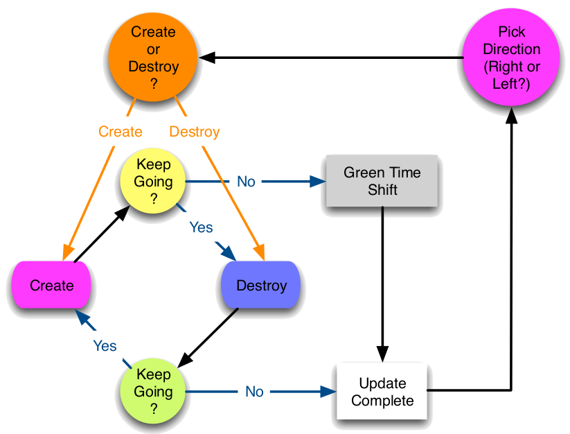
This update is said to be “directed” in imaginary time, because the Green operator has a controllable probability to perform several actions while propagating in the same direction. In order to generate configurations with the proper Boltzmann weight, all decisions during a directed update must be made with probabilities that satisfy detailed balance. A non-trivial and efficient solution for these probabilities is given in Phys. Rev. E 78, 056707 (2008). What makes the most important difference between the SGF algorithm and other algorithms is that this directed update and the proposed solution for the probabilities that satisfy detailed balance are valid for any Hamiltonian!
When the state that appears to the left of the Green operator is the same as the state that appears to the right, ψL=ψR, the Green operator acts as the identity operator. In that case the configuration of the extended partition function is also a configuration of the true partition function. This means that measurements can be performed when such a configuration occurs. All details on measurements are given in Phys. Rev. E 77, 056705 (2008).
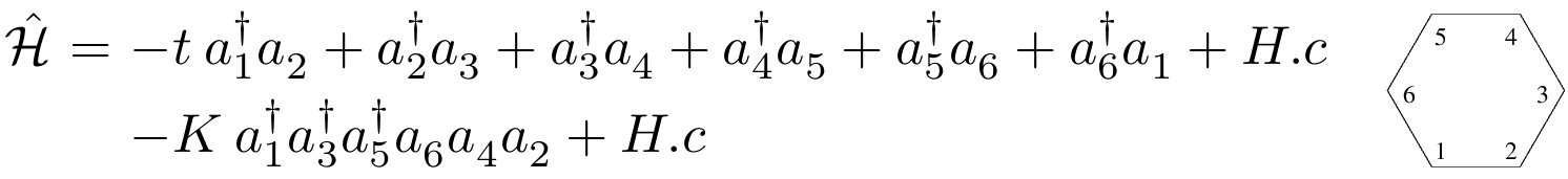
In the following examples, we consider three particles on a single hexagon with kinetic and ring-exchange terms, described by the Hamiltonian below. We represent the two imaginary time boundaries τ=0 and τ=β by purple hexagons (time increases from right to left). The Green operator is represented by a green ellipsoid, kinetic operators by red ellipsoids, and ring-exchange operators by blue stars. Each break in the animations indicates the beginning and/or the end of a directed update.
Not sure you want to subscribe? Take a peek at the description of the Blue Moonshine channel to get an idea of its contents.